|
Designing
Air Flow Systems |
|||
|
|
A theoretical
and practical guide to the basics of designing air flow systems. |
||
|
1.
Air Flow 1.1.
Types of Flow 1.2.
Types of Pressure
Losses or Resistance to Flow 1.3.
Total
Pressure, Velocity Pressure, and Static Pressure 2.
Air Systems 2.1.
Fan Laws 2.2.
Air Density 2.3.
System Constant 3.
Pressure Losses of
an Air System 3.1.
Sections in Series 3.2.
Sections in Parallel 3.3.
System Effect 4.
Fan Performance
Specification 4.1.
Fan Total Pressure 4.2.
Fan Static Pressure 5.1.
Methodology 5.2.
Assumptions and
Corrections 6.
Problem # 1 – An Exhaust System 7.
Problem # 2 – A Change to the
System’s Air Flow Rate 8.
Problem # 3 – A Supply System |
|
|
Flow of air or any other fluid is
caused by a pressure differential between two points. Flow will originate from an area of high
energy, or pressure, and proceed to area(s) of lower energy or pressure.

Duct air
moves according to three fundamental laws of physics: conservation of mass,
conservation of energy, and conservation of momentum.
Conservation of mass simply states that an air mass is neither created
nor destroyed. From this principle it follows that the amount of air mass
coming into a junction in a ductwork system is equal to the amount of air mass
leaving the junction, or the sum of air masses at each junction is equal to
zero. In most cases the air in a duct is assumed to be incompressible, an
assumption that overlooks the change of air density that occurs as a result of
pressure loss and flow in the ductwork. In ductwork, the law of conservation of
mass means a duct size can be recalculated for a new air velocity using the
simple equation:
V2 = (V1 * A1)/A2
Where V is velocity and A is Area
The law of energy conservation states that energy cannot
disappear; it is only converted from one form to another. This is the basis of
one of the main expression of aerodynamics, the Bernoulli equation.
Bernoulli's equation in its simple form shows that, for an elemental flow
stream, the difference in total pressures between any two points in a duct is
equal to the pressure loss between these points, or:
(Pressure loss)1-2 = (Total pressure)1 - (Total pressure)2
Conservation of momentum is based on
Laminar Flow
Flow
parallel to a boundary layer. In HVAC
system the plenum is a duct.
Turbulent Flow
Flow which is perpendicular and near
the center of the duct and parallel near the outer edges of the duct.
Most HVAC applications fall in
the transition range between laminar and turbulent flow.
1.2. Types of Pressure Losses or
Resistance to Flow
Pressure loss is the loss of total pressure in a duct or fitting.
There are three important observations that describe the benefits of using
total pressure for duct calculation and testing rather than using only static
pressure.
·
Only total pressure in ductwork always drops in the direction of flow.
Static or dynamic pressures alone do not follow this rule.
·
The measurement of the energy level in an air stream is uniquely
represented by total pressure only. The pressure losses in a duct are
represented by the combined potential and kinetic energy transformation, i.e.,
the loss of total pressure.
·
The fan energy increases both static and dynamic pressure. Fan ratings
based only on static pressure are partial, but commonly used.
Pressure loss in ductwork has three components, frictional
losses along duct walls and dynamic losses in fittings and component losses in
duct-mounted equipment.
Component Pressure
Due to physical items with known pressure drops, such as
hoods, filters, louvers or dampers.
Dynamic Pressure
Dynamic losses are the result of changes in direction and velocity of air
flow. Dynamic losses occur whenever an air stream makes turns, diverges,
converges, narrows, widens, enters, exits, or passes dampers, gates, orifices,
coils, filters, or sound attenuators. Velocity profiles are reorganized at these
places by the development of vortexes that cause the transformation of
mechanical energy into heat. The disturbance of the velocity profile starts at
some distance before the air reaches a fitting. The straightening of a flow
stream ends some distance after the air passes the fitting. This distance is
usually assumed to be no shorter then six duct diameters for a straight duct.
Dynamic losses are proportional to dynamic pressure and can be calculated using
the equation:
Dynamic loss = (Local loss coefficient) * (Dynamic
pressure)
where the Local loss coefficient, known as a C-coefficient,
represents flow disturbances for particular fittings or for duct-mounted
equipment as a function of their type and ratio of dimensions. Coefficients can be found in the ASHRAE Fittings
diagrams.
A local loss coefficient can be related to different
velocities; it is important to know which part of the velocity profile is
relevant. The relevant part of the velocity profile is usually the highest
velocity in a narrow part of a fitting cross section or a straight/branch
section in a junction.
Frictional Pressure
Frictional losses in duct sections are result from air viscosity and
momentum exchange among particles moving with different velocities. These losses also contribute negligible losses or gains in air systems unless there
are extremely long duct runs or there are significant sections using flex duct.
The easiest way of defining frictional loss per unit length
is by using the Friction Chart (ASHRAE, 1997); however, this chart (shown below) should be used for
elevations no higher of 500 m (1,600 ft), air temperature between 5°C and 40°C
(40°F and 100°F), and ducts with smooth surfaces. The Darcy-Weisbach Equation should be used for “non-standard” duct type such as flex
duct.
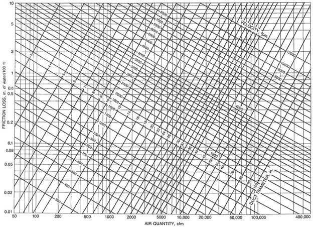
Friction Chart (ASHRAE HANDBOOK, 1997)
1.3. Total Pressure, Velocity Pressure, and Static
Pressure
It is convenient to calculate pressures in ducts using as a
base an atmospheric pressure of zero. Mostly positive pressures occur in supply
ducts and negative pressures occur in exhaust/return ducts; however, there are
cases when negative pressures occur in a supply duct as a result of fitting
effects.
Airflow through a duct system creates three types of
pressures: static, dynamic (velocity), and total. Each of these pressures can be
measured. Air conveyed by a duct system imposes both static and dynamic
(velocity) pressures on the duct's structure. The static pressure is responsible
for much of the force on the duct walls. However, dynamic (velocity) pressure
introduces a rapidly pulsating load.
Static pressure
Static pressure is the measure of the potential energy of a
unit of air in the particular cross section of a duct. Air pressure on the duct
wall is considered static. Imagine a fan blowing into a completely closed duct;
it will create only static pressure because there is no air flow through the
duct. A
balloon blown up with air is a similar case in which there is only static
pressure.
Dynamic (velocity) pressure
Dynamic pressure is the kinetic
energy of a unit of air flow in an air stream. Dynamic pressure is a function of
both air velocity and density:
Dynamic pressure = (Density) * (Velocity)2 / 2
The static and dynamic pressures are mutually convertible;
the magnitude of each is dependent on the local duct cross section, which
determines the flow velocity.
Total Pressure
Consists of the pressure the air exerts in the direction of
flow (Velocity Pressure) plus the pressure air exerts perpendicular to the
plenum or container through which the air moves. In other words:
PT = PV + PS
PT = Total Pressure
PV = Velocity Pressure
PS = Static Pressure
This general rule is used to derive what is called the Fan
Total Pressure.
See the section entitled Fan Performance Specifications for a definition
of Fan Total Pressure and Fan Static Pressure.
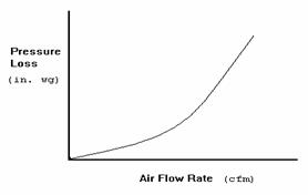
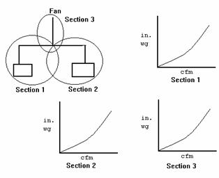
For kitchen ventilation applications an air system consists
of hood(s), duct work, and fan(s). The relationship between the air flow rate
(CFM) and the pressure of an air system is expressed as an increasing
exponential function.
The graph below shows an example of a system curve. This curve shows
the relationship between the air flow rate and the pressure of an air
system.
Complex systems with branches and junctions, duct size
changes, and other variations can be broken into sections or sub-systems. Each section or
sub-system has its own system curve. See the diagram below for an illustration of
this concept.
Use the Fan Laws along a system
curve. If
you know one (CFM, S.P.) point of a system you could use Fan Law 2 to determine
the static pressure for other flow rates. They apply to a fixed air system. Once any element of
the system changes, duct size, hood length, riser size, etc.. the system curve
changes.
CFM x RPM
x
Fan Law 1
------- =
-------
CFM known RPM known
SP x CFM2 x RPM2x
Fan Law 2
------ = ------- = -------
SP known CFM2known RPM2known
BHPx CFM3x RPM3x
Fan Law 3
------ = ------- =
-------
BHPknown CFM3known
RPM3known
Other calculations can be utilized to maneuver around a fan
performance curve.
For example, to calculate BHP from motor amp draw, use the following
formula:
1 phase motors
3 phase
motors
BHP = V * I * E * PF
BHP = V * I * E * PF * 1.73
746
746
where:
BHP = Brake Horsepower
V = Line Voltage
I = Line Current
E = Motor Efficiency (Usually about .85 to .9)
PF = Motor Power Factor (Usually about .9)
Once the BHP is known, the RPM of the fan can be
measured. The
motor BHP and fan RPM can then be matched on the fan performance curve to
approximate airflow.
The most common influences on air density are the effects
of temperature other than 70 °F and barometric pressures other than 29.92” caused by
elevations above sea level.
Ratings found in fan performance tables and curves are
based on standard air. Standard air is defined as clean, dry air
with a density of 0.075 pounds per cubic foot, with the barometric pressure at
sea level of 29.92 inches of mercury and a temperature of 70 °F. Selecting a fan to operate at conditions
other then standard air requires adjustment to both static pressure and brake
horsepower. The volume of air will not be affected in a
given system because a fan will move the same amount of air regardless of the
air density. In other words, if a fan will move 3,000 cfm at 70 °F it will also move 3,000 CFM at 250 °F. Since 250 °F air weighs only 34% of 70°F air, the fan will require less BHP but it will also
create less pressure than specified.
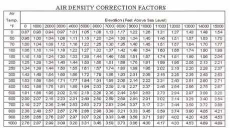
When a fan is specified for a given CFM and static pressure
at conditions other than standard, the correction factors (shown in table below)
must be applied in order to select the proper size fan, fan speed and BHP to
meet the new condition.
The best way to understand how the correction factors are
used is to work out several examples. Let’s look at an example using a
specification for a fan to operate at 600°F at sea level. This example will clearly show that the fan
must be selected to handle a much greater static pressure than specified.
Example #1:
A 20” centrifugal fan is required to deliver 5,000 cfm at 3.0 inches
static pressure. Elevation is 0 (sea level). Temperature is 600°F. At standard conditions, the fan will require
6.76 bhp
1.
Using the chart below, the correction factor is 2.00.
2.
Multiply the specified operating static pressure by the correction factor
to determine the standard air density equivalent static pressure. (Corrected static
pressure = 3.0 x 2.00 = 6”. The fan must be selected for 6 inches of
static pressure.)
3.
Based upon the performance table for a 20 fan at 5,000 cfm at 6 inches
wg, 2,018 rpm is needed to produce the required performance.
4.
What is the operating bhp at 600 °F?
Since the horsepower shown in the performance chart refers
to standard air density, this should be corrected to reflect actual bhp at the
lighter operating air.
Operating bhp = standard bhp ¸ 2.00 or 6.76 ¸ 2.00 = 3.38 bhp.
Every air system or sub-system has a system constant. This constant can
be calculated as long as you know one (CFM, Static Pressure) point. You use a
variation of the fan laws to calculate the system constant. To calculate the
system constant:
K system = S.P./(CFM)2
Once you have the system constant you can calculate the
static pressure for any flow rate.
S.P. = (CFM)2 * K system
3. Pressure Losses of an Air
System
Pressure losses are more easily determined by breaking an
air system into sections. Sections can be in series or in parallel.
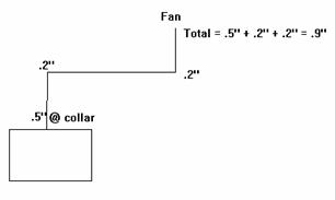
For sections or components in series simply sum up all the
sections. A single duct that has the same shape, cross section, and
mass flow is called a duct section or just a section.
Following is the recommended procedure for calculating total
pressure loss in a single duct section:
·
Gather input data: air flow, duct shape, duct size,
roughness, altitude, air temperature, and fittings;
·
Calculate air velocity as a function of air flow and cross
section;
·
Calculate local C-coefficients for each fitting used; and
·
Calculate pressure loss using the friction
chart
The following is a simple example of how duct pressure
accumulates and is totaled in a section.
When designing sections that are parallel it is important
to remember that
the branches of a junction all have the same total pressure. This is a
fact. It is
governed by a principle which states that areas of high energy move to areas of lower
energy. We
will see how this applies to air systems in parallel.
To illustrate these concepts we will reference the diagram
below. In this
example we calculate the pressure losses for Section 1 to be -0.75” at the
junction. We
calculate the pressure losses for Section 2 to be -0.6” at the junction. (NOTE:
For simplicity’s sake we do not consider the pressure loss incurred by the
junction.)
These would be the actual pressure losses of the system were they
operating independently; however, they do not. They interact at the junction. This means that
whenever air flow encounters a junction it will take the path of least
resistance and the total pressure losses of each branch of the junction will be
the same.
For sections that run parallel, always use the
section with the higher pressure loss/gain to determine pressure
losses/gains through a system. Adjust the branch with the lower pressure
loss/gain by increasing the flow rate or decreasing the duct size to increase
the pressure loss to that of the higher branch.
If the flow rate or the duct size is not changed the air
flow through each branch will adjust itself so that each branch has the same
total pressure loss/gain. In other words, more air flows through the
branch with the lower pressure loss/gain or energy state.
In the example below, the actual pressure loss would be
somewhere between -0.75” and -0.6”. Section 1 would pull less than 2000 CFM and
Section 2 would pull more than 1800 CFM. 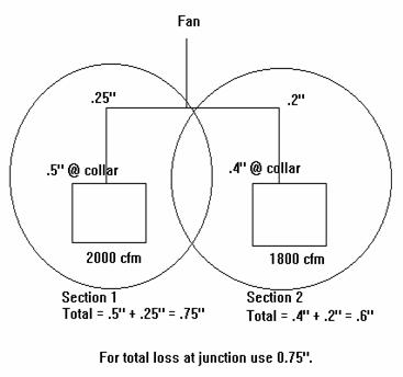
3.3. System Effect
System Effect occurs in an air system when two or more
elements such as fittings, a hood and a fitting, or a fan and a fitting occur
within close proximity to one another. The effect is to increase the energy or
pressure in a system as air flows through the elements. To calculate the
pressure loss incurred by such a configuration, consider two elements at a
time. For
example, if two elbows occur 4 feet from one another this configuration will
have a pressure loss associated with it.
Calculate the pressure loss/gain associated with each
fitting as if it occurs alone. Sum these and multiply them by a system
effect coefficient (K). The system effect coefficient can be obtained
from the ASHRAE Fitting Diagrams for only a limited number of configurations of
elements.
Configurations not listed must use estimates or best
guesses. In
many cases, you can use a listed configuration as a guide.
One configuration not listed is an elbow within close
proximity to the collar of a hood. As a rule of thumb, the chart below can offer
some guidance for determining the system effect for this situation. Remember the
coefficients in the chart are only an estimate.
|
Distance between Riser and Elbow |
System Effect Coefficient (K) |
|
2 feet |
1.75 |
|
3 feet |
1.5 |
|
4 feet |
1.3 |
|
5 feet |
1.2 |
The diagrams below show system effect factors for straight
through elements and turning elements. For rectangular ductwork, D =
(2HW)/(H+W).
The following formula should be used to calculate the pressure caused by
system effect:
Pressure Loss = K * (Element A Resistance + Element B
Resistance)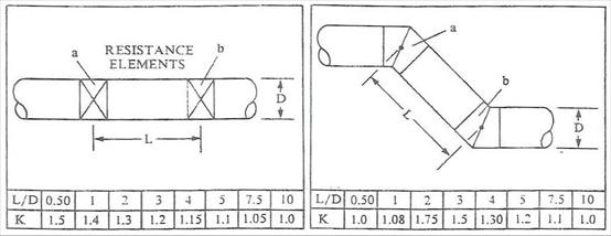
Straight Through Flow
Turning
Elements
The following diagrams show proper and improper methods of
constructing ductwork:
4. Fan Performance
Specification
A fan performance spec is given as a Fan Total Pressure
or a Fan Static
Pressure which can handle a certain flow rate. Most manufacturers'
performance charts are based on Fan Static Pressure.
Fan total Pressure is the pressure differential between the
inlet and the outlet of the fan. It can be expressed in these terms:
P t fan = P t loss + P v system outlet + (P s system outlet + P s system entry + P v system entry)
P
t fan = Fan Total Pressure
P t loss = Dynamic, Component, and Frictional Pressure through the
air system.
P
s system outlet = Static Pressure at System Outlet
P
s system entry = Static Pressure at System Entry
P
v system entry = Velocity Pressure at System Entry
P v system outlet = Velocity Pressure at System
Outlet
For most HVAC applications: (P s outlet + P s entry + P v entry) = 0
Therefore:
P
t fan = P t loss + P v system outlet
The Fan Static Pressure is expressed as the Fan Total
Pressure minus the velocity pressure at the fan discharge, or:
P s fan = P t loss + P v system outlet - P v discharge
Where P v discharge = Velocity Pressure at the Fan Discharge.
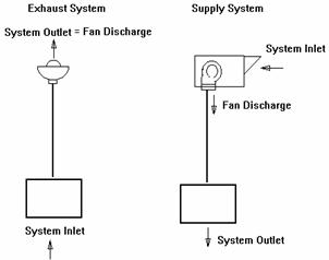
For Exhaust Systems with resistance only on the inlet
side, the fan static pressure is:
P s fan = P t loss
For exhaust system: P v system outlet = P v discharge
For Supply Systems with resistance on the outlet side, the
fan static pressure is:
P s fan = P t loss - P v discharge
P v system outlet can be
assumed to be 0.
The diagram below illustrates the difference between
exhaust and supply systems.
Break the system into sections.
A new section occurs at:
1) Changes in duct size.
2)
Change in air volume
Calculate losses for each section.
Begin at the section farthest from the fan and work towards the fan.
For each
section:
1.
Write down or calculate all known variables.
Air Flow Rate. (Q)
Duct Cross-Sectional Area of the section. (A)
Center-Line Length of the section. (L)
Air Velocity through the section. (V=Q/A)
Velocity Pressure. (Pv =
(V/4005)2)
2.
Write down or calculate all pressure losses in the section.
a) List the Component
Losses/Gains.
Incurred by hoods, ESPs, filters, dampers, etc..
b) Calculate the Dynamic
Losses/Gains.
Occur through elbows, transitions, tees, or any other type of
fitting.
Use the ASHRAE Fitting Diagrams to find Dynamic Loss Coefficients for
fittings.
Be sure to factor in System Effect!
c) Calculate Frictional
Losses/Gains.
Use the ASHRAE Friction Chart for “standard” galvanized ductwork.
Use the Darcy-Weisbach Equation for “non-standard” duct such as flex
duct.
3.
Sum up the Component, Dynamic, and Frictional Pressure for
the section.
4.
Sum up the pressure losses for all of the sections.
5.2. Assumptions and
Corrections
Standard Air Density, .075 lb/cu ft, is used for most HVAC
applications.
Frictional losses based on galvanized metal duct with 40
joints per 100 ft.
Correction for "Non-Standard" Duct Material
If material other than galvanized metal is used in parts of
the system, you will have to adjust for the difference in the material's
roughness factor.
This means the Friction Chart typically used to determine frictional
losses cannot be used and you must use a variation of the Darcy-Weisbach
Equation.
See the section titled Equations for more information on this equation.
Correction for Density
Not needed if the temperature is between 40 °F to 100 °F and
elevations are between 1000 ft to 1000 ft.
Correction for Moisture
Not needed if air temperature < 100 °F.
6. Problem # 1 – An
Exhaust System
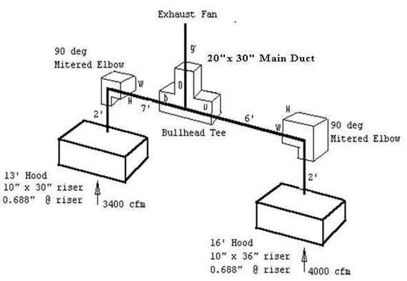
The first step is to break the system into sections.
Section 1 runs from the 16’ Hood to the Bullhead Tee.
Section 2 runs from the 13’ Hood to the Bullhead Tee.
Section 3 runs from the Bullhead Tee to the Exhaust Fan.
Now calculate the pressure losses for each section.
Section 1
Air Flow Rate Q = 4000 cfm
Cross-Sectional Area A = 10 x 36/144 = 2.5 ft2
Center Line Distance L = 2’ + 6’ = 8’
Velocity V = 4000/2.5 = 1600 ft/min
Velocity Pressure = Pv1 = (V/4005)2 = (1600/4005)
2 = 0.16”
Loss Calculations
Component Losses
Hood Loss
Phood1 = -0.688”
Look up from manufacturer hood static pressure curves. Here is a link to
the Hood Static
Pressure Calculator.
Frictional Losses
Use the Friction Chart to look up the pressure loss per 100 ft
of duct.
Pfr1 = -(.16”/100 ft) * (8’) = -0.013”
Dynamic Losses
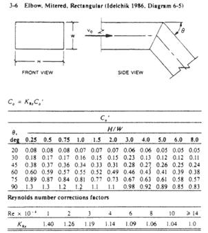
Mitered
Elbow. Look up Fitting 3-6 in Appendix 2 -
ASHRAE Fittings.
The dynamic coefficient C0 = 1.3
Pelbow1 = - Pv1 = -(1.3)*(0.16”) = -0.208”
Bullhead
Tee.
Look up coefficient from Appendix 3 - Bullhead Tee Curves.
Some general rules for bullhead tees:
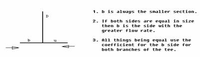
Since Section 1 has a larger duct size, this section is the
“u“ side of the
bullhead tee. The following describes how to use the
bullhead tee curves to find Ku for the “u“ side of the
bullhead tee.
Since AU /AD = (10x36)/(20x30) = .6, we find the bullhead tee
curves for which AU /AD is .6 and the y-axis represents KU.
We know that Qb /QD =
4000/(4000+3400) = .54. For simplicity and ease of graphing, we round
.54 to the nearest 10th giving us .5.
We also know that Ab /AD = (10x30)/(20x30) = .5.
Equipped with these ratios, can draw a line from the point
on the x-axis where Qb /QD is .5 up to where it intersects the curve for which
Ab /AD is .5
We find Ku = 1.6
NOTE: Due to human error resulting from manually graphing
the value of KU , the number you graph may be
slightly different than the value show above. The important thing is to know how to use the
curves and get a reasonable value for KU.
Now we can calculate the pressure drop contributed by the
bullhead tee for Section 1:
Pbulltee1 = -Ku * Pv1 =
-(1.6)*(0.16”) = -0.256”
The total pressure loss for Section 1 is:
P t loss 1 = Phood1 + Pfr1 + Pelbow1 + Pbulltee1
P t loss 1 = -0.688” -0.013” -0.208” -0.256” =
-1.165”
Section 2
Air Flow Rate Q = 3400 cfm
Cross-Sectional Area A = 10 x 30/144 = 2.1 ft2
Center Line Distance L = 2’ + 7’ = 9’
Velocity V = 3400/2.1 = 1619 ft/min
Velocity Pressure = Pv2 = (V/4005)2 = (1619/4005)
2 = 0.16”
Loss Calculations
Component Losses
Hood Loss
Phood2 = -0.688”
Look up from hood static pressure curves.
Frictional Losses
Use the Friction Chart to look up the pressure loss per 100 ft
of duct.
Pfr2 = -(.18”/100 ft) * (9’) = -0.016”
Dynamic Losses
Mitered Elbow. Look up Fitting 3-6 in Appendix 2 -
ASHRAE Fittings.
The dynamic coefficient C0 = 1.3
Pelbow2 = - Pv2 = -(1.3)*(0.16”) = -0.208”
Bullhead Tee. Using the methodology described for the
bullhead tee in Section 1, we can find the value of the coefficient, Kb, for the “b“ side of the bullhead tee. Use the bullhead tee
curves for which AU /AD is .6 and the y-axis represents Kb.
We find that Kb = 1.75 and the resulting
pressure loss is:
Pbulltee 2 =
-Kb * Pv2 =
-(1.75)*(0.16”) = -0.280”
The total pressure loss for Section 2 is:
P t loss 2 = Phood2 + Pfr2 + Pelbow2 + Pbulltee2
P t loss 2 = -0.688” -0.016” -0.208” -0.280” =
-1.192”
Balance by Design
Note that the pressure loss of Section 2 is greater than
the loss of Section 1. To balance the system by design increase the
air flow rate in Section 1 to bring it up to the higher pressure loss of Section
2.
To correct the air flow rate for Section 1 use the Fan Laws:
Q 1 new = Q 1 old * (P t loss 1 new/ P t loss 1 old)1/2
Q 1 new = 4000 * (1.192/1.165)1/2 = 4046 cfm
Section 3
Air Flow Rate Q = 3400 cfm + 4046 cfm = 7446 cfm
Cross-Sectional Area A = 20 x 30/144 = 4.17 ft2
Center Line Distance L = 9’
Velocity V = 7446/4.17 = 1785 ft/min
Velocity Pressure = Pv3 = (V/4005)2 = (1785/4005)
2 = .20”
Loss Calculations
Component Losses
None
Frictional Losses
Use the Friction Chart to look up the pressure loss per 100 ft
of duct.
Pfr2 = -(.15”/100 ft) * (9’) = -0.014”
Dynamic Losses
None
Total pressure loss for Section 3 is:
P t loss 3 = Pfr3
P t loss 3 = -0.014”
Total Pressure Loss of System
Since the pressure loss of Section 2 is greater than that
of Section 1, it is used to calculate the pressure loss of the entire system as
shown below:
P t loss = P t loss 2 + P t loss 3 = -1.192” -0.014” =
-1.206”
7. Problem # 2 – A Change in the System’s Air
Flow Rate
Now we will change the air flow rate through Section 2 from
3400 CFM to 3000 CFM.
We will illustrate how once you know one (CFM, S.P.) point of a system
you can use the Fan Laws to calculate the pressure loss for other air flow
rates.
Section 1
There is no change. P t loss 1 = -1.165”
Section 2
Air Flow Rate Q = 3000 CFM
Cross-Sectional Area A = 10 x 30/144 = 2.1 ft2
Center Line Distance L = 2’ + 7’ = 9’
Velocity
V =
3000/2.1 = 1429 ft/min
Velocity Pressure = Pv2 = (V/4005)2 = (1429/4005)
2 = 0.13”
Loss Calculations
Component Losses
Hood Loss. Use the Fan Laws to calculate a new
Hood Loss or look it up in the Hood S.P. chart.
Phood2 =
-(0.688”)*((3000 CFM)2/(3400 CFM)2)
Phood2 = -0.536”
Frictional Losses
Use the Friction Chart to look up the pressure loss per 100 ft
of duct.
Pfr2 = -(.15”/100 ft) * (9’) = -0.014”
Dynamic Losses
Mitered
Elbow. Look up Fitting 3-6 in Appendix 2 -
ASHRAE Fittings.
The dynamic coefficient C0 = 1.3
Pelbow2 = - Pv2 = -(1.3)*(0.13”) = -0.169”
Bullhead Tee. Since Section 2 is the “b” side, we use
the set of bullhead tee curves for which AU
/AD is .6 and the y-axis represents Kb.
We find that Kb = 1.65
Pbulltee 2 =
-Kb * Pv2 =
-(1.65)*(0.13”) = -0.215”
Total Section Loss:
P t loss 2 = Phood2 + Pfr2 + Pelbow2 + Pbulltee2
P t loss 2 = -0.536” -0.014” -0.169” -0.215” =
-0.93”
Using the Fan Laws to calculate the new total
pressure loss for Section 2:
P t loss 2 = -(1.192”)*((3000 CFM)2/(3400 CFM)2) =
-0.93”
Balance by Design
Note that the pressure loss of Section 1 is now greater
than the loss of Section 2. To balance the system by design we must
increase the air flow rate in Section 2 to bring it up to the higher pressure
loss of Section 1.
To correct the air flow rate for Section 2 use the Fan Laws:
Q 2 new = Q 2 old * (P t loss 2 new/ P t loss 2 old)1/2
Q 2 new = 3000 * (1.165/0.93)1/2 = 3357 CFM
Section 3
Air Flow Rate Q = 3357 CFM + 4000 CFM = 7357 CFM
Cross-Sectional Area A = 20 x 30/144 = 4.17 ft2
Center Line Distance L = 9’
Velocity V = 7357/4.17 = 1764 ft/min
Velocity Pressure = Pv3 = (V/4005)2 = (1764/4005)
2 = 0.19”
Loss Calculations
Component Losses
None
Frictional Losses
Use the Friction Chart to look up the pressure loss per 100 ft
of duct.
Pfr2 = -(0.14”/100 ft) * (9’) = -0.013”
Dynamic Losses
None
Using the Fan Laws to calculate the new total
pressure loss for Section 3:
P t loss 3 = -(0.014”)*((7357 cfm)2/(7446 cfm)2) =
-0.013”
Total System Loss
Calculated with Tables and ASHRAE Charts
P t loss = P t loss 1 + P t loss 3 = -1.165” -0.013” =
-1.178”
As shown above, Branch 1 of the junction is used to
calculate the system’s total pressure loss because it has the greater pressure
drop of the two branches.
Calculated with the Fan Laws
P t loss = -(1.206”)*((7357 cfm)2/(7446 cfm)2) = -1.178”
8. Problem # 3 - A Supply
System
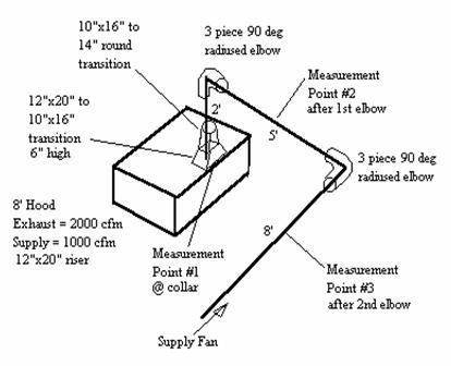
The first part of the problem will show the pressure gains
obtained from measuring the total pressure at 3 points shown in the diagram
above. It will
provide some rules of thumb for estimating pressure for elbow and at the supply
collar. The
second part of the problem will calculate the pressure gain of the system and
compare it to the measured pressure gain.
The entire system satisfies the definition of a section
since there are no junctions or duct size changes. The transitions off
the supply collars can be included in the section.
Supply System - Measured Pressure
A 0” to 1” Dwyer manometer was used to measure the pressure
of the system at 3 points. The pressure was measured for two different
flow rates.
The results are show in the table below.
Measurements Taken at 3 points of the Supply System
|
Air Flow Rate (CFM) |
Velocity (ft/min) |
Point 1 @ collar (in. wg) |
Point 2 after 1st elbow (in. wg) |
Point 3 after 2nd elbow (in. wg) |
|
1000 |
935 |
0.075 |
0.140 |
0.260 |
|
1920 |
1793 |
0.276 |
0.570 |
0.910 |
The table shows:
1)
How high air velocities greatly increase the pressure. When the air flow
rate is raised to 1920 cfm, the velocity through the duct about doubles and the
pressure increases 3-1/2 fold.
2)
The system effect of having 2 elbows close to each other and being close to the hood.
Using the pressure gains for 1000 cfm flowing through the
system, we see that the pressure gain for the first elbow is: 0.14” - 0.075” =
0.065”. This
reflects the system effect of having an elbow close to the supply opening of a
hood.
The pressure gain for the second elbow is: 0.26” - 0.14” =
0.12”. This
reflects the system effect of having two elbows within close proximity to one
another and being close to the hood.
3)
When the system supplies 1000 CFM, the pressure gain at the supply collar is 0.075”. This illustrates
how low the pressure really is when a system is designed for the desired
velocity between 900 and 1000 ft/min. The table below provides some rules of thumb
when estimating pressure gain at the supply collar:
|
Hood Length (L) |
Pressure Loss Estimate |
|
L <= 8’ |
1/16” max. |
|
8’ < L <= 12’ |
1/16” to 1/8” max. |
|
12 < l <= 16’ |
1/8” to 1/4” max. |
This table assumes that the system has been designed for velocities
around 1000 ft/min.
Test Kitchen Supply System - Calculated Pressure
Section 1
Air Flow Rate Q = 1000 cfm
Cross-Sectional Area A = pr2 = p (7)2/144 = 1.069 ft2
Center Line Distance L = 15’
Velocity V = 1000/1.069= 935 ft/min
Velocity Pressure = Pv1 = (V/4005)2 = (935/4005) 2
= 0.055”
Loss Calculations
Component Losses
Hood.
Assume 1/16” pressure gain at the collar.
P hood = 0.063”
Frictional Losses
Use the Friction Chart to look up the pressure loss per 100 ft
of duct.
Pfr = -(0.095”/100 ft) * (15’) = 0.014”
Dynamic Losses
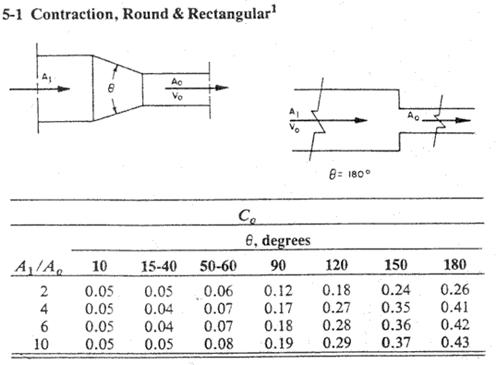
12”x 20” to 10” x 16” Rectangular Transition
Use ASHRAE fitting 5-1 in Appendix 2 – ASHRAE
Fittings.
To find the dynamic coefficient we calculate:
q/2 = tan -1(2”/6”) = 18o Therefore: q = 36 o
A0 / A1 =
(12x20)/(10x16) = 1.5
Therefore C0 = 0.05
P trans1 = C0Pv1 = (0.05)(0.055”) = 0.003”
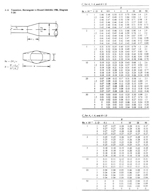
10”x 16” Rectangular to 14” Round Transition
Use ASHRAE fitting 4-6 in Appendix 2 – ASHRAE
Fittings.
B = W/H(A0 / A1 )2 =
(16/10)(1.069/1.111)2 = 1.48
Re = 8.56DV = (8.56)(14”)(935 ft/min) = 11205
Therefore Re x 10-4 = 11. Use the value for Re x 10-4 = 10
L/D is not relevant in this case.
C0 = 0.11
P trans2 = C0Pv1 = (0.11)(0.055”) = 0.006”
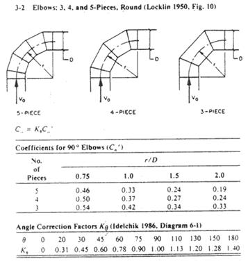
Two 90 o Radius Elbows
Use ASHRAE fitting 3-2. Assume a 3 piece elbow.
Assume r = 10”. So, r/D = 10/14 = .71 therefore Kq = 1.
C0 = 0.54
P elbow1 = C0Pv1 = (0.54)(0.055”)
= 0.03”
P elbow2 = C0Pv1 = (0.54)(0.055”)
= 0.03”
We must figure in the system effect incurred by having an
elbow close to the supply collar. Use the table in the System Effect section of
this paper to estimate the system effect.
The elbow is about 2’ above the supply riser to KSE = 1.75.
P SE elbow-hood = KSE P elbow1 =
(1.75)(0.03”) = 0.053”
Now we must factor in the system effect for the 2 elbows in
succession. We
decide to the S-Shaped fitting in the ASHRAE handbook to estimate the system
effect. We use
ASHRAE
fitting 3-14.
q = 90 o
L/D = 60”/14” = 4.29
K SE = 1.55
P SE S-fitting = K SE(P elbow1 + P elbow2) = 1.55(0.03” + 0.03”) = 0.093”
Total Section Loss:
P t loss 1 = Phood + Pfr + Ptrans1 + Ptrans2 + P SE
elbow-hood + P SE
S-fitting
P t loss 1 = 0.063” + 0.014” + 0.003” + 0.006” +
0.053” + 0.093”
P t loss 1 =
0.232”
The measured value of 0.26” differs because of error in the system effect
estimates.
Now we can determine the size fan we need. A 10” blower will handle 1000 cfm at
0.232”.
To calculate the Fan Static Pressure:
P
s fan = P t loss - P v discharge
Use the blower manufacturer product literature to get the
dimensions for the blower outlet so the velocity pressure at the fan discharge
can be calculated:
P v discharge = (V discharge/4005)2
P v discharge = ((1000/((11.38*13.13)/144))/4005)2
P v discharge = 0.058”
P
s fan = 0.232” - 0.058” = 0.174”
Total Pressure (P T)
P T = P v + P s
P
v = Velocity Pressure
P s = Static Pressure
Fan Static Pressure (P s fan)
For Exhaust:
P s fan = P t loss
For Supply:
P s fan = P t loss - P v discharge
P s fan = Fan Static Pressure
P t loss = Dynamic and Friction Losses
P
v discharge = Velocity Pressure at the Fan Discharge
Velocity Pressure (P v)
P v = r(V/1097)2
For standard air P v equals:
P v = (V/4005)2
V = Velocity through the duct.
Friction Losses (P fr)
Darcy-Weisbach Equation
P
fr = (f / D) x L x VP
Then substitute (f / D) with H f:
P fr = Hf x L x VP
L = Duct Section Length (ft)
f = Friction Factor
D = Duct Diameter (ft)
H f is defined as:
H f = aVb / Qc
V = Velocity through the duct
cross section.
Q = Flow Rate (cfm) through the duct section.
See Table titled Surface Roughness Correlation Constants to get values
for a,b, and c.
Surface Roughness Correlation Constants
|
Material |
k |
A |
b |
c |
|
Aluminum, Black Iron, Stainless Steel |
0.00015 |
0.0425 |
0.0465 |
0.602 |
|
Galvanized |
0.0005 |
0.0307 |
0.533 |
0.612 |
|
Flexible Duct |
0.003 |
0.0311 |
0.604 |
0.639 |
k = Roughness factor for the material.
10. Appendix 2 – ASHRAE
Fittings
Fitting 3-2
Fitting 3-6
11. Appendix 3 – Bullhead Tee Curves
Au/Ad = 0.2, Kb
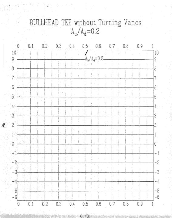
Au/Ad = 0.2, Ku
Au/Ad = 0.3, Kb
Au/Ad = 0.3, Ku
Au/Ad = 0.4, Kb
Au/Ad = 0.4, Ku
Au/Ad = 0.5, Kb
Au/Ad = 0.5, Ku
Au/Ad = 0.6, Kb
Au/Ad = 0.6, Ku
Au/Ad = 0.8, Kb
Au/Ad = 0.8, Ku
Au/Ad = 1.0, Kb
Au/Ad = 1.0, Ku